Recently, I’ve had some spare time to go back through some material from the end of college that I didn’t think I’d quite mastered (thanks covid!). One of these topics is the Gaussian Mixture model and how we can use expectation maximization to implement it.

Gaussian Mixture Models and E&M

Gaussian mixture models are a class of probabilistic unsupervised learning algorithms. A GMM assumes that the process that generated the data can be described by a finite number of Gaussian distributions with unknown parameters. The learning problem is then to find those parameters. This can be done via maximum likelihood estimation (MLE). The concept of MLE is to maximize some likelihood function so that given an assumed model, the observed data is most probable. From a Bayesian standpoint, MLE is equivalent to maximum a posteriori (MAP) with a uniform prior.

The simplest algorithm to do MLE iteratively is expectation maximization. It consists of two steps the (E)xpectation step and the (M)aximization step. In the E step, the expected value of the log likelihood function is calculated. The M step then chooses parameters to maximize the function calculated in the E step. This process is then repeats until convergence.

More detail on the theory behind these can be found in Bishop’s Pattern Recognition and Machine Learning, the psudocode from which I try to follow as close as I can.

Implementation

I tried to keep the implementation as straightforward as possible.

def GaussianMixtureModel(X, k = 2, max_iters = 10000, eps = 1e-3):
    # I followed the psudocode on Bishop p 438-439 as close as I could
    # select initial means randomly
    means = X[np.random.randint(0,len(X),k)] 
    # initiate responsibilities
    respons = np.zeros((X.shape[0], k))
    # initiate mixing coeffs pi_k
    mix = np.ones(k)
    # hardest part: getting correct shape here
    # I used the shape returned by sklearn.mixture._estimate_gaussian_covariances_full
    # which does an initial M step for the cov as well, but I didn't
    covs = np.full((k, X.shape[1], X.shape[1]),
                   np.cov(X.T))

    log_likelihoods = [0]
    for i in range(max_iters):  
        # E step
        llh , respons = E(X, k, mix, means, covs, respons)
        # M step
        mix, means, covs, respons = M(X,k, mix, means, covs, respons)
        # stop when the likelihood doesnt change with error eps
        if np.abs(llh - log_likelihoods[-1]) <= eps:
            return means, respons, mix, covs, log_likelihoods
        # note down log likelihoods for learning curve
        log_likelihoods.append(llh)

    print("Max Iterations Exceeded")
    return means, respons, mix, covs, log_likelihoods
    
def log_likelihood(respons):
    ret = 0
    for i in range(len(respons)):
        ret += np.log(np.sum(respons[i]))
    return ret

def E(X, K, mix, means, covs, respons):
    # calc the llh and re-evaulte the responsibilities
    for k in range(K):
        # Bishop 9.23
        # easier to split up fraction and normalize later
        respons[:, k] = mix[k] * multivariate_normal(means[k], covs[k]).pdf(X)
    llh = log_likelihood(respons)
    respons /= respons.sum(axis = 1, keepdims = True)
    return llh, respons

def M(X, K, mix, means, covs, respons):
    # re-estimate params using current responsibilities
    # define N_k as rowwise sum of responsibilities
    # Bishop 9.27
    N_k = respons.sum(axis = 0)
    # Bishop 9.24
    means = respons.T@X / N_k # recalc means
    for k in range(K): # recalc variances
        # Bishop 9.25
        covs[k] = (respons[:, k] * (X - means[k]).T@(X - means[k])) / N_k[k]
    mix = N_k/len(respons) # Bishop 9.26
    return mix, means, covs, respons

Now let’s test our code on some generated data.

mu_x = np.array([5,10])
mu_z = np.array([6,11])

sig_x = np.zeros(2)+ 0.01
sig_z = np.zeros(2)+ 0.05

X = multivariate_normal.rvs(mu_x, sig_x, size = 100)
Z = multivariate_normal.rvs(mu_z, sig_z, size = 100)

plt.scatter(*X.T)
plt.scatter(*Z.T)

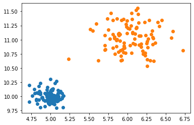
We’ve generated two different clusters, each with a different underlying distribution. Let’s try to run our model and see if it can correctly find the parameters of the distributions.

dat = np.vstack((X,Z))
means, respons, weights, covs, log_likelihoods = GaussianMixtureModel(dat)
print(means)
print(covs)

[[ 4.99037355 9.99691058]

[ 6.03674847 11.03166029]]

[[[ 0.01063869 -0.00127132]

[-0.00127132 0.0099645 ]]

[[ 0.05877937 0.00100672]

[ 0.00100672 0.05401486]]]

We appear to be quite close. Let’s visualize the 1,2,3 sigma contours.

def plt_contours(X, preds, means, covs,
                 minx = -500, maxx = 800,
                 miny = -500, maxy =  5000):
    t = np.linspace(minx, maxx, 100)
    h = np.linspace(miny, maxy, 100)

    w_0, w_1 = np.meshgrid(t,h)
    z = multivariate_normal(means[0],covs[0]).pdf(np.dstack((w_0, w_1)))
    plt.contour(t, h, z, levels = 3)
    z = multivariate_normal(means[1],covs[1]).pdf(np.dstack((w_0, w_1)))
    plt.contour(t, h, z, levels = 3)
    plt.scatter(*X.T, c = preds)
    plt.show()

preds = np.argmax(respons, axis = 1)
plt_contours(dat, preds, means, covs,
                 minx = 4, maxx = 7,
                 miny = 9, maxy =  12)
                 

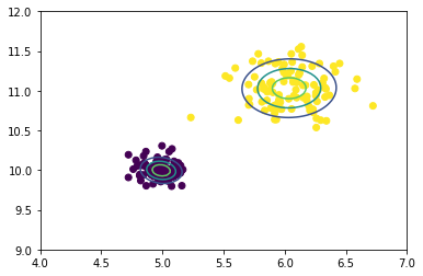
As you can see, the contour bands are about where we could expect, as we know the variance in the purple cluster is quite small compared to the yellow cluster. I’d call this a success!

I’m sure the code could be made a bit faster, but sklearn’s implementation exists for production, so I opted for clarity. Anyway, thanks for reading and hopefully this toy implementation/example was useful.